Blog

  • Data-oriented design and CPU caches

    Data-oriented design and CPU caches

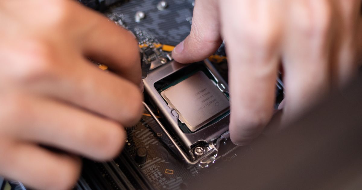
    The single biggest performance lesson I ever learned is that modern CPUs are not slow at computing, they are slow at waiting for memory. A cache miss to main memory can cost a couple hundred cycles. In that time the CPU could have done hundreds of additions. Once you internalize that gap, you start designing programs around how data moves, not just what operations run on it. That is the heart of data-oriented design.

    The memory hierarchy is the real machine

    Between the CPU and main memory sit several layers of cache: L1 is tiny and nearly as fast as registers, L2 is bigger and slower, L3 bigger and slower still. When the CPU needs a byte, it does not fetch one byte. It fetches a whole cache line, typically 64 bytes, and stores it in cache. If your next access is within that line, it is nearly free. If it is somewhere far away, you pay the full miss penalty.

    This means the layout of your data in memory directly controls your performance. Two programs doing the identical arithmetic can differ by an order of magnitude based purely on access patterns.

    Arrays of structs versus structs of arrays

    The classic example is how you store a collection of records. The intuitive object-oriented layout is an array of structs:

    struct Particle {
        float x, y, z;     // position
        float vx, vy, vz;  // velocity
        float mass;
        char name[32];
    };
    struct Particle particles[100000];
    
    // update positions
    for (int i = 0; i < 100000; i++) {
        particles[i].x += particles[i].vx;
    }

    This loop only touches x and vx, but every cache line it loads is full of mass, name, and the other fields you do not need. You are dragging cold data through cache for nothing. The data-oriented layout splits the fields into parallel arrays, a struct of arrays:

    struct Particles {
        float x[100000], y[100000], z[100000];
        float vx[100000], vy[100000], vz[100000];
        float mass[100000];
    };
    
    for (int i = 0; i < 100000; i++) {
        p.x[i] += p.vx[i];
    }

    Now the x array and vx array are each densely packed. Every byte you pull into cache is a byte you use. On real hardware this kind of change routinely gives 3x to 10x speedups on hot loops, with no algorithmic change at all.

    Why pointer chasing hurts

    Linked lists and node-based trees are the opposite of cache-friendly. Each node is a separate heap allocation that can live anywhere, so traversing the list jumps all over memory and misses the cache on nearly every step. If you understand stack vs heap memory and how heap allocations scatter, this follows naturally. A flat array you scan linearly is dramatically faster than a linked list with the same number of elements, even though both are O(n), because the hardware prefetcher can predict and preload sequential access.

    • Prefer contiguous arrays over node-based structures when you iterate often.
    • Group fields you access together, and separate the ones you do not.
    • Process data in the order it sits in memory whenever you can.
    • Keep hot data small so more of it fits in cache at once.

    It is the same idea as a good allocator

    This is why allocation strategy matters so much. If you allocate ten thousand objects one at a time, they end up scattered. If you allocate them in one block, they sit together and iterate fast. The custom allocator in writing a simple memory allocator gives you exactly this control: you decide the layout instead of leaving it to chance.

    False sharing, the multicore trap

    There is a nastier cache effect that shows up with threads. If two cores each write to different variables that happen to live in the same 64 byte cache line, the hardware has to keep bouncing that line between their caches even though the threads never touch the same bytes. This is called false sharing, and it can quietly destroy the scaling of an otherwise parallel program. The fix is to pad or align the per-thread data so each thread's hot variables sit on their own cache line. I have seen a loop go from no speedup on eight cores to near linear scaling with nothing more than a padding field added to a struct.

    When to reach for this

    I do not restructure everything around the cache. For code that runs once or rarely, clarity wins. But for the hot loops, the inner kernels that run millions of times, data layout is usually the first thing I tune and often the highest return. Profile first, find where the cache misses are, then lay the data out the way the hardware wants to read it. The machine is happy to be fast if you stop making it wait.


  • Database schema best practices

    Database schema best practices

    The schema is the part of a system that is hardest to change once it is full of data. You can rewrite a service in a weekend. Migrating a billion-row table without downtime is a project. So I spend real time on the schema up front, because the cost of getting it wrong only grows. These are the decisions I do not regret.

    Let the database enforce the rules

    Application code is not the place to guarantee data integrity, because there is always another path in: a migration script, a manual fix, a second service, a developer in a console. The database is the one chokepoint everything passes through, so that is where the rules belong. I use NOT NULL aggressively, foreign keys to enforce relationships, unique constraints to prevent duplicates, and check constraints for value ranges.

    CREATE TABLE orders (
      id          bigint GENERATED ALWAYS AS IDENTITY PRIMARY KEY,
      customer_id bigint NOT NULL REFERENCES customers(id),
      status      text   NOT NULL DEFAULT 'pending'
                  CHECK (status IN ('pending','paid','shipped','cancelled')),
      total_cents integer NOT NULL CHECK (total_cents >= 0),
      created_at  timestamptz NOT NULL DEFAULT now()
    );

    Every constraint here is a bug that can never reach production. A status of “shippd” gets rejected at write time instead of breaking a report three weeks later.

    Normalize first, denormalize on evidence

    I start normalized: each fact lives in exactly one place. Duplicated data is duplicated truth, and the copies drift apart the moment someone updates one and forgets the other. Normalization keeps writes simple and correctness cheap.

    Denormalization is a performance optimization, and like any optimization I want a measurement before I do it. When a specific query is genuinely too slow and the profile points at joins, then I will cache a computed value or duplicate a column, knowing I am taking on the job of keeping the copies in sync. Doing it preemptively is how you get a schema full of fields nobody trusts.

    Choose keys and types deliberately

    Every table gets a synthetic primary key, usually a bigint identity or a UUID. I avoid natural keys like email addresses as primary keys, because the one thing you can promise about a natural key is that it will change, and changing a primary key that is referenced everywhere is misery. Use types that mean something:

    • Store money as integer cents, never floats. Floating point and currency are old enemies.
    • Always use timestamp-with-time-zone for time, and store UTC.
    • Reach for a native enum or a check constraint instead of free-text status fields.
    • Use the database’s real JSON type for genuinely unstructured data, not a text blob.

    Index for your reads, but know the cost

    An index makes reads fast and writes slightly slower, and it takes space. I index foreign keys, columns I filter on regularly, and columns I sort by. I do not index everything, because an unused index is pure overhead on every insert. The way to know is to look: most databases will tell you which indexes go untouched, and those are candidates for removal.

    Composite indexes are worth understanding because column order matters. An index on (customer_id, created_at) helps a query filtering by customer and sorting by date, but it does nothing for a query that only filters by date. The same observability mindset I described in logging and observability best practices applies here: measure the real query patterns before you guess.

    Treat migrations as code

    Every schema change goes through a migration file, checked into version control, reviewed like any other change. No manual ALTER statements run by hand in production, ever, because the next environment will not have them and you will spend a day chasing the difference. The same review discipline from code review best practices applies, with extra care, since a bad migration can lock a table or drop data.

    • Make migrations forward-only and additive where you can. Add a column, backfill, then later remove the old one in a separate step.
    • Avoid changes that take a long exclusive lock on a large, live table.
    • Test the migration against a copy of production-sized data before you run it for real.

    A schema you can evolve safely is worth more than a perfect schema you are afraid to touch. Build for change, because change is the only certainty.

  • Publishing a Flutter app to the App Store and Play Store

    Publishing a Flutter app to the App Store and Play Store

    Writing the app is half the job. Getting it into both stores is the other half, and it is the half that surprises people. Apple and Google each have their own signing, their own metadata, and their own review moods. I have shipped through both more times than I can count, and the difference between a smooth release and a stressful one is preparation. Here is the path I follow.

    Set the basics before you build

    Before you generate a single release binary, get the boring fields right. A unique application id that you will never change, a sensible version and build number, the app name, and the minimum supported OS versions. Changing the application id after launch is effectively a new app, so decide it carefully. These live in the Gradle config on Android and the Xcode project on iOS.

    # pubspec.yaml controls the version and build number
    version: 1.0.0+1
    # 1.0.0 is the version users see, +1 is the build number

    Android signing and the app bundle

    Google Play wants an app bundle rather than an APK now, and it wants it signed with an upload key you create once and guard carefully. Lose that key and you are in for a painful recovery process. I store the keystore outside the repository and reference it through a properties file that is never committed. Building the release bundle is a single command once signing is wired up.

    flutter build appbundle --release
    # produces build/app/outputs/bundle/release/app-release.aab

    Upload that file to the Play Console, fill in the store listing, set up the content rating questionnaire, and choose a release track. I always push to internal testing first so I can install the exact artifact users will get before it goes public.

    iOS signing and archiving

    Apple signing is more involved. You need an Apple Developer account, certificates, an app id, and provisioning profiles. Xcode can manage most of this automatically if you sign in, which I recommend over wrangling profiles by hand. You build the iOS release through Flutter and then archive and upload through Xcode or the transporter tool.

    flutter build ipa --release
    # then open Xcode, archive, and upload to App Store Connect
    • Register the app id in the developer portal
    • Let Xcode manage certificates and profiles where possible
    • Upload to TestFlight before submitting for review
    • Prepare screenshots for every required device size

    Store listings take longer than you think

    Both stores need screenshots at specific sizes, an icon, a description, keywords, a privacy policy URL, and a data collection disclosure. Apple is strict about the privacy questionnaire and will reject vague answers. Set aside real time for this, because a half done listing blocks the whole release. I keep a checklist so nothing gets missed at the last minute.

    Surviving review

    Apple review can reject for reasons that feel arbitrary until you read the guidelines closely. The common ones are missing demo account credentials, broken links, crashes on their test device, and unclear use of permissions. Give them a working login if your app needs one, test on a real device, and explain why you ask for each permission. Google review is usually faster and more automated but still cares about permissions and policy compliance.

    Plan the updates too

    Shipping version one is the start. Bump the build number every upload, keep a changelog, and use staged rollouts on Android so a bad release reaches a small slice of users first. The performance habits from Flutter performance optimization matter here because crash and jank metrics affect your store ranking. And if your app leans on native features, test those carefully across OS versions as I describe in Flutter platform channels. A calm release is a prepared release. Do the boring work early and launch day stops being scary.

  • How to optimize images for the web

    How to optimize images for the web

    If a page feels slow, images are the first thing I check, and they are almost always the culprit. Text and code are tiny. A single uncompressed hero photo can outweigh your entire JavaScript bundle. The good news is that image optimization is mostly mechanical, and you can automate the whole thing.

    Choose the right format

    Format choice is the highest-leverage decision you make. JPEG is fine for photographs but it is old and inefficient. PNG is for images that need transparency or sharp edges, like logos and screenshots, and it is terrible for photos. The modern answer for almost everything is WebP, which gives you JPEG-quality photos at a fraction of the size, and AVIF when you want to push compression even further. I serve AVIF with a WebP fallback and a JPEG fallback below that.

    • Photographs: AVIF or WebP, never raw JPEG if you can avoid it.
    • Logos and icons: SVG when possible, it scales infinitely and weighs nothing.
    • Screenshots with text: PNG or WebP lossless so the text stays crisp.

    Resize before you compress

    This is the mistake I see constantly. People take a 4000 pixel wide camera photo, compress it, and display it in a 600 pixel column. The browser downloads all those wasted pixels and throws them away. Resize the image to the largest size it will actually be shown at first, then compress. Resizing alone often cuts file size by 80 percent before you have touched quality settings.

    To know the right target width, look at how wide the image actually renders in your layout, then double it for high-density screens. A photo shown at 600 pixels should be exported at 1200 so it stays crisp on a retina display, and no larger. Going beyond that is pure waste, because the extra pixels never reach a single eye. I keep a small table of the render widths in my design and resize to match each one.

    Automate it with sharp

    I do not hand-edit images in an app. I run them through a script using the sharp library, which is fast and produces excellent output. A short pipeline resizes and converts everything in a folder:

    const sharp = require('sharp');
    
    sharp('input.jpg')
      .resize({ width: 1200, withoutEnlargement: true })
      .webp({ quality: 75 })
      .toFile('output.webp')
      .then(() => console.log('done'));

    Quality 75 on WebP is my default. The difference between 75 and 90 is invisible on a screen but doubles the file size. Drop it into your build and every image gets the same treatment automatically, which fits neatly into a pipeline run through CI/CD with GitHub Actions.

    Serve responsive sizes

    A phone and a desktop should not download the same image. Generate a few widths and let the browser pick using srcset. The markup tells the browser what sizes exist and how wide the image renders, and it grabs the smallest one that still looks sharp:

    <img
      src="photo-800.webp"
      srcset="photo-400.webp 400w, photo-800.webp 800w, photo-1200.webp 1200w"
      sizes="(max-width: 600px) 100vw, 600px"
      alt="A descriptive caption"
    >

    Lazy load everything below the fold

    Add loading="lazy" to images that are not visible when the page first paints. The browser then defers loading them until the user scrolls near. This is a one-attribute change with a big payoff, because it stops offscreen images from competing for bandwidth with the content people actually see. Leave it off your hero image though, since you want that one to load immediately.

    Always set width and height

    Set explicit width and height attributes, or a CSS aspect ratio, on every image. Without them the browser does not know how much space to reserve, so the page jumps around as images load. That jump is layout shift, and it is one of the metrics Google grades you on. It also just feels broken to users. Reserving the space costs nothing and fixes it completely.

    The payoff

    Put these together and a typical image-heavy page goes from several megabytes to a few hundred kilobytes with no visible quality loss. That shows up directly in your load times and your Core Web Vitals. Lighter images mean a snappier site everywhere, including the moment you push it live through Cloudflare Pages and your visitors load it from the edge. Optimize once in the build, and you never have to think about it per-image again.

  • Database design and normalization (and when to denormalize)

    Database design and normalization (and when to denormalize)

    I have inherited enough broken schemas to have strong opinions. The worst outages I have dealt with were almost never about a missing index or a slow disk. They were about a data model that lied. A column that meant three different things depending on the row. A “status” field that was secretly a free-text dumping ground. A foreign key that existed in someone’s head but never in the database. Good design is the cheapest insurance you will ever buy, and you buy it before you write a single query.

    This post is about how I actually approach normalization, what the normal forms buy you in practice, and the handful of situations where I deliberately denormalize. If you want the requirements-gathering side of this, I wrote that up separately in my data modeling methodology guide. This one is about the schema itself.

    What normalization actually protects you from

    People talk about normalization like it is an academic exercise. It is not. Every normal form exists to prevent a specific class of bug that will eventually wake you up at 3am. Strip away the formal language and the goal is simple. Store each fact exactly once, in the place where it belongs, so that there is no way for two copies of the same fact to disagree.

    When the same piece of data lives in two places, those two places will drift apart. Not maybe. They will. Someone updates the customer’s email in one table and forgets the other. A batch job touches half the rows. Now you have two truths and no way to know which one is correct. Normalization removes the second copy so the contradiction becomes impossible rather than merely unlikely.

    The normal forms, the way I think about them

    I do not walk around quoting the formal definitions, but I do keep their intent in my head when I sketch tables.

    • First normal form means no repeating groups and no multi-valued columns. If you find yourself naming columns phone1, phone2, phone3, you have a separate table waiting to be born. A comma-separated list in a varchar is the same crime wearing a disguise.
    • Second normal form means every non-key column depends on the whole primary key, not just part of it. This only bites you with composite keys, but when it bites it leaves a mark.
    • Third normal form means non-key columns depend on the key and nothing but the key. If a column depends on another non-key column, it belongs in its own table. The classic example is storing a city and its postal code together when one determines the other.

    In day to day work, if I hit third normal form I am usually in good shape. Boyce-Codd and the higher forms matter for specific overlapping-key situations, but third normal form catches the vast majority of real modeling mistakes I see in code review.

    A concrete example

    Say we are storing orders. The naive version crams everything into one wide table, repeating the customer name and email on every single order row. Here is the normalized version I would actually ship.

    -- Customers own their own facts, once
    CREATE TABLE customers (
        id          BIGINT GENERATED ALWAYS AS IDENTITY PRIMARY KEY,
        email       CITEXT NOT NULL UNIQUE,
        full_name   TEXT NOT NULL,
        created_at  TIMESTAMPTZ NOT NULL DEFAULT now()
    );
    
    -- Orders reference the customer, they do not copy it
    CREATE TABLE orders (
        id           BIGINT GENERATED ALWAYS AS IDENTITY PRIMARY KEY,
        customer_id  BIGINT NOT NULL REFERENCES customers(id),
        status       TEXT NOT NULL
                     CHECK (status IN ('pending','paid','shipped','cancelled')),
        placed_at    TIMESTAMPTZ NOT NULL DEFAULT now()
    );
    
    -- Line items are their own grain: one row per product per order
    CREATE TABLE order_items (
        order_id     BIGINT NOT NULL REFERENCES orders(id),
        product_id   BIGINT NOT NULL REFERENCES products(id),
        quantity     INT NOT NULL CHECK (quantity > 0),
        unit_price   NUMERIC(12,2) NOT NULL,
        PRIMARY KEY (order_id, product_id)
    );

    Notice a few choices that are not strictly about normal forms but travel with good design. The status column has a CHECK constraint so the database itself enforces the allowed values. The unit_price lives on the line item, not on the product, because the price at the moment of sale is a different fact from the current price. That distinction is the kind of thing normalization forces you to think about. Is this the current value or the value as it was? They are not the same fact and they do not belong in the same column.

    Constraints are part of the design, not decoration

    A schema without constraints is a suggestion. I push as much invariant enforcement into the database as I reasonably can, because application code is the wrong place to guarantee data integrity. There will always be a second writer eventually. A migration script, an admin tool, a coworker poking around in a psql session. The database is the only layer all of them share.

    So I use NOT NULL aggressively, foreign keys without apology, UNIQUE constraints on anything that should be unique, and CHECK constraints for value ranges and enumerations. If you only take one habit from this post, make it this one. Most of the “mysterious bad data” I have debugged would have been impossible with a constraint that took thirty seconds to write. I go deeper on this in my notes on schema best practices.

    When I denormalize on purpose

    Now the heresy. I denormalize regularly, and I do not feel bad about it, because denormalization done with intent is an optimization, not a mistake. The trick is that you only denormalize after you understand the access pattern, never before. Premature denormalization is just a data model with extra bugs.

    Here are the cases where I reach for it.

    • Read-heavy aggregates. If a dashboard reads an order total a thousand times for every one time the order changes, computing that total on every read is wasteful. I will store a cached total column and keep it current with a trigger or in the same transaction as the write.
    • Reporting and analytics tables. Transactional normalization and analytical query patterns pull in opposite directions. A wide, denormalized table or a star schema can turn a brutal eight-way join into a single scan. I keep these separate from the source of truth and rebuild them from it.
    • Expensive joins on the hot path. Sometimes a join is genuinely the bottleneck even after indexing. Copying one frequently-read column to avoid a join can be worth it, as long as you own the update path.

    The non-negotiable rule with every one of these is that the normalized version remains the source of truth. The denormalized copy is derived, disposable, and rebuildable. The moment you have two independent sources of truth you are back to the original sin that normalization existed to prevent.

    How I keep denormalization safe

    If I store a derived value, I make the derivation explicit and I make it automatic. A cached column gets updated in the same transaction as its source, or by a trigger, never by a hopeful comment that says “remember to update this.” A materialized view gets a documented refresh schedule. A reporting table gets rebuilt by a job I can run on demand and verify against the source.

    I also write a check, even a slow one I run nightly, that compares the derived value against a fresh computation and screams if they disagree. Drift is the failure mode of denormalization, and the only defense is to detect it early. Once you can prove the copy matches the source, the performance win comes with a clear conscience. When the copies do start to disagree, it is almost always because a query plan changed or an index disappeared, which is exactly the territory I cover in my indexing deep dive.

    The order I do things in

    My default sequence has not changed in years. Normalize first, to third normal form, with real constraints. Get it correct and let it be correct. Then measure. Only when a specific, measured access pattern demands it do I introduce a denormalized copy, and only as a derived artifact with an enforced update path. Correctness first, then speed, and never speed bought with a lie in the data.

    That order matters because it is far easier to denormalize a clean model than to clean up a model that was muddy from birth. Start strict. Loosen deliberately. Your future self, paged at 3am, will thank you.

  • A practical data modeling methodology, from requirements to schema

    A practical data modeling methodology, from requirements to schema

    Almost every truly painful schema I have had to live with started the same way. Someone opened a migration file and started typing CREATE TABLE before anyone had agreed on what the data actually was. The tables came first and the understanding came later, which is exactly backwards. A schema is the last artifact in modeling, not the first. By the time I write SQL, the hard thinking is already done.

    This is the methodology I use to get from a fuzzy feature request to a schema I am willing to sign my name to. It is not heavy. It does not need special tooling. It mostly needs you to slow down for an afternoon so you can move fast for the next two years. For the design principles that govern the final schema, pair this with my post on normalization and when to denormalize.

    Step one, gather the nouns and the rules

    I start by reading or listening to how the people who actually do the work describe it. Not the engineers. The people in the domain. I am hunting for two things. The nouns, which become candidate entities, and the rules, which become constraints and relationships.

    When a logistics coordinator says “a shipment can have many parcels but every parcel belongs to exactly one shipment,” they have just handed me a one-to-many relationship and a NOT NULL foreign key, for free, in plain language. The domain experts are doing the modeling already. My job is to write it down faithfully and notice when their sentences contradict each other.

    I keep a running glossary as I go. The single most underrated modeling tool is an agreed definition of each term. When two people use the word “account” to mean two different things, you will not find out until production, unless you forced the definition early.

    Step two, find the entities and their identity

    From the nouns, I pull out the real entities. The test I apply is identity. Does this thing have an existence of its own that I need to refer to over time? A customer does. An order does. A line on an order does. The color “blue” usually does not, it is an attribute, until the day the business needs a color catalog with its own rules, at which point it earns entity status.

    For every entity I ask one question immediately. What makes a row unique? Sometimes there is a natural key, like an ISO country code. More often there is not, and I add a surrogate key, a generated identity column with no business meaning. I lean toward surrogate keys for most entities because natural keys have a nasty habit of changing, and a primary key that changes is a primary key that ruins your week.

    Step three, map the relationships

    Now I connect the entities, and I am precise about cardinality because cardinality is where the schema is decided.

    • One to many is the common case. The “many” side carries a foreign key pointing back to the “one” side. An order has many items, so order_items carries the order_id.
    • Many to many always becomes a junction table. There is no other honest way to represent it. Students and courses meet in an enrollments table that carries both foreign keys.
    • One to one is rare and deserves suspicion. Usually it means you either have one entity that you split for no reason, or you have an optional extension that genuinely belongs in its own table. I make myself justify every one-to-one.

    For each relationship I also pin down the participation rules. Is the foreign key mandatory or optional? What should happen on delete? These are not afterthoughts. ON DELETE behavior is a real business decision dressed up as a technical one, and the business should get a vote.

    Step four, attributes and the grain question

    With entities and relationships in place, I attach attributes, and for each one I ask what it really is. Is it atomic, or is it secretly several facts crammed together? A “name” field that everyone wants to search by first and last name is two columns pretending to be one. An address is almost always several.

    The most important question at this stage is grain. What does one row in this table represent, exactly, in one sentence? If I cannot say it cleanly, the table is confused and the queries will be too. “One row per order” is a clear grain. “One row per order, except sometimes per shipment” is a future incident report.

    Step five, write the schema and let the database help

    Only now do I write SQL, and at this point it almost writes itself, because the thinking is finished. Here is the kind of thing that falls out of the steps above for a simple course enrollment domain.

    -- One row per student
    CREATE TABLE students (
        id          BIGINT GENERATED ALWAYS AS IDENTITY PRIMARY KEY,
        email       CITEXT NOT NULL UNIQUE,
        full_name   TEXT NOT NULL,
        enrolled_on DATE NOT NULL DEFAULT CURRENT_DATE
    );
    
    -- One row per course offering
    CREATE TABLE courses (
        id        BIGINT GENERATED ALWAYS AS IDENTITY PRIMARY KEY,
        code      TEXT NOT NULL UNIQUE,     -- natural key, stable per catalog
        title     TEXT NOT NULL,
        capacity  INT NOT NULL CHECK (capacity > 0)
    );
    
    -- The junction table: one row per student per course
    CREATE TABLE enrollments (
        student_id BIGINT NOT NULL REFERENCES students(id) ON DELETE CASCADE,
        course_id  BIGINT NOT NULL REFERENCES courses(id)  ON DELETE RESTRICT,
        grade      TEXT CHECK (grade IN ('A','B','C','D','F') OR grade IS NULL),
        PRIMARY KEY (student_id, course_id)
    );

    Look at how much of the model is now enforced by the database rather than left to hope. The many-to-many becomes a composite primary key, which also prevents a student from enrolling twice in the same course without any application code. The two different ON DELETE choices encode a real rule: deleting a student removes their enrollments, but you cannot delete a course that still has students in it.

    Step six, validate against the queries you will run

    A model is only as good as the questions it can answer. Before I call it done, I take the five or ten queries the application will actually run most often and I write them against the schema on paper. If a common question requires a tortured five-table join or a subquery nested three deep, the model is fighting the workload and I go back a step.

    This is also where access patterns start to inform indexing, though I keep that as a separate concern. Get the model honest first, then make it fast. I walk through the performance side in detail in my database indexing deep dive.

    Step seven, plan for change

    No model survives contact with a roadmap unchanged, so I design for evolution from the start. I avoid columns that mean different things in different rows. I prefer adding a nullable column or a new table over overloading an existing one. I keep a migration discipline where every schema change is a versioned, reviewable file, never a manual edit to a live database.

    The mindset that has served me best is this. Modeling is the act of writing down what is true about the world, carefully enough that the database can enforce it. The SQL is just the transcript. Do the thinking first, write the schema last, and validate it against the real questions, and you end up with tables that feel boring in the best possible way. Boring schemas do not page you.

  • How pointers really work

    How pointers really work

    Pointers scared me for an embarrassingly long time. The syntax did not help: asterisks meaning two different things, ampersands, arrows. But the concept is simple once you strip the syntax away. A pointer is a variable whose value is a memory address. That is it. It is a number that tells you where something lives.

    Memory is one giant array

    Picture your process’s address space as one enormous array of bytes, indexed from zero up to some huge number. Every variable you declare lives at some index in that array. A pointer just stores one of those indices. When you “dereference” a pointer, you are saying “go to that index and read what is there.”

    int x = 42;
    int *p = &x;      // p holds the address of x
    printf("%d\n", *p);   // dereference: prints 42
    *p = 7;           // write through the pointer
    printf("%d\n", x);    // prints 7

    The ampersand means “address of” and the asterisk in an expression means “the thing at this address.” The same asterisk in a declaration means “this variable is a pointer.” Two different jobs for one symbol, which is the main reason pointers look confusing at first.

    The type matters more than you think

    A pointer is not just an address, it is an address plus a type. The type tells the compiler two things: how many bytes to read when you dereference, and how far to jump when you do arithmetic. An int pointer and a char pointer can hold the exact same numeric address and behave completely differently.

    int arr[4] = {10, 20, 30, 40};
    int *p = arr;     // points at arr[0]
    p++;              // now points at arr[1], moved 4 bytes not 1
    printf("%d\n", *p);   // prints 20

    That is the key insight about pointer arithmetic. Adding one to an int pointer moves it by sizeof(int) bytes, not by one byte. The compiler scales for you based on the type. This is also why arrays and pointers feel so interchangeable in C: indexing arr[i] is defined as taking the address of arr, adding i times the element size, and dereferencing.

    Where pointers point

    A pointer can hold the address of a stack variable, a heap allocation, a function, or nothing at all. The where matters because it decides whether dereferencing is safe. If you are fuzzy on stack versus heap lifetimes, that is the foundation here, and I covered it in stack vs heap: how memory actually works. A pointer to a stack variable becomes dangling the moment that frame returns. A pointer to freed heap memory is a use-after-free waiting to crash.

    • NULL pointer: holds address zero, a deliberate “points at nothing.” Dereferencing it crashes, which is actually the friendly outcome.
    • Dangling pointer: holds an address that used to be valid. Dereferencing it is undefined behavior and may silently corrupt data.
    • Wild pointer: never initialized, holds garbage. The worst kind because it can point anywhere.

    Pointers to pointers

    Once a pointer is just a variable, a pointer to a pointer stops being mysterious. It is the address of a variable that itself holds an address. You need this whenever a function must change where a pointer points, not just what it points to.

    void allocate(int **out) {
        *out = malloc(sizeof(int));   // write a new address into the caller's pointer
        **out = 99;                   // write a value into that memory
    }
    
    int *p = NULL;
    allocate(&p);     // pass the address of p so the function can modify it
    printf("%d\n", *p);   // prints 99

    const and what is really protected

    One thing that trips people up is where const sits relative to the asterisk, because a pointer has two things that can be constant: the address it holds, and the data it points at. A const int pointer means you cannot change the data through it, but you can repoint it. A pointer that is itself const means you can change the data but not where it points. Reading the declaration right to left helps. This matters because the compiler will enforce it, and getting it wrong produces error messages that look more confusing than the underlying idea.

    Why this is worth the trouble

    Pointers are the mechanism behind almost everything interesting in systems code: linked structures, dynamic memory, passing large objects without copying them, talking to hardware at fixed addresses. They are also the source of most crashes in C. The allocator I describe in writing a simple memory allocator is nothing but careful pointer manipulation over a raw block of bytes. Once you see a pointer as a typed integer into the big byte array, the fear goes away and the power shows up.

  • Vector databases explained: embeddings and similarity search

    Vector databases explained: embeddings and similarity search

    The first time I shipped a feature backed by a vector database, I spent an afternoon confused about why my results made no sense. I had treated it like a keyword index. It is not one. A vector database stores meaning, or at least a numerical approximation of meaning, and it answers a different kind of question than the databases I had used for years. This post is the explanation I wish someone had handed me before I started.

    What an embedding actually is

    An embedding is a list of floating point numbers that represents a piece of content. You take some text, an image, or an audio clip, run it through a model, and out comes a fixed length array. A typical text embedding might have 384, 768, or 1536 dimensions. Each number on its own means nothing you can interpret. Together they place the content at a specific point in a high dimensional space.

    The useful property is that similar content lands in nearby positions. The sentence “my laptop will not turn on” and the sentence “my computer is dead” produce vectors that sit close together, even though they share almost no words. A keyword search would miss that connection entirely. An embedding captures it because the model that produced the vectors learned, from enormous amounts of text, that those phrases mean roughly the same thing.

    This is the whole trick. We convert the fuzzy human notion of “these two things are about the same topic” into a geometry problem. Once it is geometry, a computer can solve it fast.

    How similarity is measured

    Closeness in this space is usually measured with cosine similarity or, equivalently for normalized vectors, dot product. Cosine similarity looks at the angle between two vectors and ignores their length. Two vectors pointing in the same direction score near 1.0, vectors at right angles score near 0, and opposite vectors score near -1.0. Some systems use Euclidean distance instead, which measures straight line distance. The choice depends on how the embedding model was trained, and getting it wrong quietly degrades your results.

    Here is the part that surprises people coming from relational databases. There is no exact match. Every query returns a ranked list of approximately relevant items with a score attached. You decide where to cut the list off. That mental shift, from “the row that matches” to “the rows that are most similar,” is the single biggest adjustment.

    Generating embeddings in practice

    You rarely train an embedding model yourself. You call one. Here is a small example that turns a few sentences into vectors and measures how close they are.

    from sentence_transformers import SentenceTransformer
    import numpy as np
    
    model = SentenceTransformer("all-MiniLM-L6-v2")
    
    sentences = [
        "my laptop will not turn on",
        "my computer is dead",
        "what time does the store close",
    ]
    
    vectors = model.encode(sentences, normalize_embeddings=True)
    
    def cosine(a, b):
        return float(np.dot(a, b))
    
    print("laptop vs computer:", cosine(vectors[0], vectors[1]))
    print("laptop vs store:", cosine(vectors[0], vectors[2]))
    

    Run that and the first pair scores high while the second pair scores low. The model never saw these exact sentences during training. It learned the relationships from context, and that generalization is what makes the whole approach work.

    Why you need a specialized database

    You could store vectors in a normal column and compare your query against every row. That is called a brute force or exact search, and it works fine up to maybe a hundred thousand vectors. Past that it falls apart, because comparing one query against ten million vectors on every request is too slow for anything interactive.

    Vector databases solve this with approximate nearest neighbor indexes. The most common is HNSW, which stands for Hierarchical Navigable Small World. It builds a layered graph where each vector links to its neighbors, and a query walks the graph instead of scanning everything. You trade a tiny bit of accuracy for an enormous speed gain. Other index types like IVF and product quantization make different tradeoffs between memory, speed, and recall.

    • Recall is the fraction of the true nearest neighbors your index actually returns. You tune it up or down depending on how much latency you can spend.
    • Latency is how long a query takes. HNSW typically answers in single digit milliseconds even over millions of vectors.
    • Memory matters because HNSW graphs are large. Quantization shrinks vectors at some cost to precision.

    Metadata filtering is where it gets real

    Pure similarity search is rarely enough on its own. In real applications you want “find documents similar to this query, but only from this user’s workspace, written in the last 90 days.” That means combining vector search with traditional filters on metadata. How well a database handles this combination, called filtered or hybrid search, is one of the things I care about most when I evaluate options, and it is a major theme in my notes on choosing a vector database.

    Done badly, filtering forces the engine to either scan everything or return too few results because the filter eliminated most of the candidates the index found. Done well, the filter is applied during the graph traversal so you still get fast, accurate results inside the subset you care about.

    A mental model that holds up

    I think of a vector database as a search engine for meaning rather than words. A keyword index answers “which documents contain these tokens.” A vector index answers “which documents are about the same thing as this query.” Those are complementary, not competing, which is why the strongest systems I have built use both at once and merge the rankings.

    The embeddings carry the semantics. The index makes search fast at scale. The metadata filters keep results relevant to the actual user. Once those three pieces clicked for me, the rest of the field stopped feeling like magic and started feeling like engineering.

    Where this leads

    The reason vector databases exploded in popularity is that they are the storage layer underneath retrieval augmented generation. When you want a language model to answer questions about your own documents, you embed those documents, store the vectors, and retrieve the relevant ones at query time. I walk through that entire pattern in building RAG systems with vector databases, and it builds directly on everything here. If you want the broader picture of how this fits into shipping real systems, my write up on practical AI engineering covers the surrounding decisions.

    Start by generating a few embeddings and printing the similarity scores yourself. Seeing related sentences score high and unrelated ones score low does more to build intuition than any diagram. Everything else is detail on top of that one idea.

  • Practical AI engineering: shipping LLM features that hold up

    Practical AI engineering: shipping LLM features that hold up

    There is a wide gap between a demo that works in front of an audience and a feature that survives real users for a month. I have shipped a few LLM features now, and almost everything I learned the hard way lives in that gap.

    The demo is the easy 80 percent

    Wiring up a model and getting a good answer takes an afternoon. The remaining work is everything that happens when the input is weird, the model is confidently wrong, or the user asks something you never tested. That part takes the other three weeks, and it is the part that decides whether anyone keeps using the thing.

    So plan for it. Budget more time for evaluation and guardrails than for the happy path, because the happy path mostly builds itself.

    RAG: retrieval is the hard part, not generation

    Most useful LLM features need your data, not just the model’s training. Retrieval-augmented generation is the standard answer: find the relevant chunks, put them in the prompt, let the model answer from them. Simple to describe, fiddly to get right.

    The quality of a RAG system is almost entirely the quality of its retrieval. If you fetch the wrong chunks, no amount of prompt cleverness saves you. Spend your time on chunking strategy, on whether you actually need embeddings or whether plain keyword search wins for your data, and on measuring whether the retrieved context contains the answer before you ever look at the generation step.

    One concrete tip: log the retrieved chunks for every query in development. Half my RAG bugs were obvious the moment I saw what the retriever actually pulled.

    You cannot improve what you do not measure

    “It seems better” is not a metric. Before you tune anything, build a small evaluation set: thirty to fifty real inputs with known good outputs. Run it on every change. It feels like overkill until the day a prompt tweak that “obviously improved things” quietly broke a third of your cases.

    Evals do not need to be fancy. A spreadsheet of inputs, expected behavior, and a pass or fail you check by eye beats no evals at all. Automate it later once you know what you are measuring.

    Treat the model output as untrusted

    This is the lesson that connects to security. Model output is just text, and if you feed it into a database query, a shell command, or another system, it can do damage the same way user input can. If an agent reads untrusted content, that content can carry instructions, which is the prompt-injection problem I cover in agentic AI in cybersecurity.

    Validate structured output against a schema. Never pass raw model text into anything that executes. The same “input is hostile” mindset from my developer security checklist applies directly to what comes out of the model, not just what goes in.

    Cost and latency are product decisions

    The biggest model is rarely the right default. A smaller model that answers in 400 milliseconds often beats a larger one that takes four seconds, because users feel latency immediately and judge quality slowly. Cache aggressively. Route easy queries to cheap models and save the expensive one for the hard cases.

    Pick your model tier on purpose. I default to the most capable model while building, then drop down once I know which calls actually need the horsepower.

    Where this leaves you

    Shipping AI features is mostly normal engineering with a probabilistic component bolted on. The model is the fun part and the smallest part. Retrieval, evaluation, validation, and the plumbing around it are the job. If you are building the surrounding system from scratch, the patterns in modern full-stack architecture are where the model actually has to live.

  • Getting started with Flutter for Android and iOS

    Getting started with Flutter for Android and iOS

    I came to Flutter after years of maintaining separate Android and iOS codebases that drifted apart no matter how disciplined the team was. One framework, one language, two stores. That promise sounded too good, so I shipped a real app with it before deciding. It held up. Here is how I get a project running and what I wish someone had told me on day one.

    Installing the toolchain

    The install is heavier than people admit. You need the Flutter SDK, but you also need a full Android Studio install for the Android SDK and an emulator, and on a Mac you need Xcode plus the command line tools for iOS. Skip any of those and you only get half the platform. After installing, run the doctor command and fix every warning before writing a line of code.

    flutter doctor -v
    flutter create my_app
    cd my_app
    flutter run -d all

    The doctor command is the most useful thing in the SDK. It checks your Android licenses, your Xcode setup, your CocoaPods version, and whether a device is connected. I run it whenever something behaves strangely, because nine times out of ten the problem is environmental rather than in my code.

    Understanding the widget tree

    Everything in Flutter is a widget. Padding is a widget. Alignment is a widget. This feels absurd for the first week and then it clicks. Instead of setting properties on a view, you wrap widgets in other widgets, and the nesting describes your layout. The framework rebuilds parts of the tree when state changes, and it is fast because it diffs against the previous tree rather than touching the native views directly.

    import 'package:flutter/material.dart';
    
    void main() => runApp(const MyApp());
    
    class MyApp extends StatelessWidget {
      const MyApp({super.key});
    
      @override
      Widget build(BuildContext context) {
        return MaterialApp(
          home: Scaffold(
            appBar: AppBar(title: const Text('Hello')),
            body: const Center(child: Text('Running on both platforms')),
          ),
        );
      }
    }

    StatelessWidget is for things that never change after they are built. The moment you need a counter, a toggle, or any value that updates, you reach for StatefulWidget or a proper state solution. I cover that in detail in my post on Flutter state management, because picking the right approach early saves a painful refactor later.

    Hot reload changes how you work

    Hot reload is the feature that sold me. You save a file and the running app updates in under a second while keeping its current state. Tweaking a color, adjusting padding, fixing a layout bug becomes a tight loop with no rebuild. There is a difference between hot reload, which preserves state, and hot restart, which throws state away and reruns from scratch. When the UI looks wrong after a reload, a hot restart usually clears it.

    • Hot reload: keeps app state, injects changed code, near instant
    • Hot restart: resets state, slower, needed after changing top level code
    • Full rebuild: needed after changing native config or adding plugins

    Handling both platforms honestly

    One codebase does not mean you can ignore the platforms. iOS users expect a back swipe and a certain feel for scrolling. Android users expect material ripples and a hardware back button. Flutter gives you both design languages, Material and Cupertino, and you can branch on the platform when it matters. I keep this branching small and centralised so it does not spread through the whole app.

    import 'dart:io' show Platform;
    import 'package:flutter/material.dart';
    
    Widget adaptiveSpinner() {
      if (Platform.isIOS) {
        return const CupertinoActivityIndicator();
      }
      return const CircularProgressIndicator();
    }

    Project structure I settle on

    The default template dumps everything in one file. That is fine for a demo and terrible for an app you maintain. I split code into folders by feature rather than by type, so a feature owns its screens, its models, and its logic in one place. This pays off the day you delete a feature and want it gone cleanly.

    Once you have the structure, the next things to worry about are how the app talks to native APIs and how it stays smooth under load. I dig into native bridges in Flutter platform channels, and into keeping frame times low in Flutter performance optimization. Get the foundation right first, then layer those concerns on top.

    What to build first

    Do not start with your dream app. Build something small that touches a network call, a list, a detail screen, and local storage. That covers most of what a real app needs and exposes the rough edges of your setup while the stakes are low. By the time you have done that twice, the framework stops fighting you and starts disappearing into the background, which is exactly where a good tool belongs.